Neural Net Optimization, Part 2 — PyTorch Writ Small
The second in a four-part series on neural network optimization, focusing on PyTorch fundamentals and how to implement PyTorch on a per neuron level.
Fine-Grained PyTorch: What Does a Neuron Really Learn?
In Part 1, we fit a third-order polynomial equation to build a computational graph. Here in Part 2, we’ll see what a single PyTorch neuron can do.
The Single PyTorch Linear Neuron
A single linear neuron in PyTorch fits functions of the form:
\[y = w x + b\]This function produces a first-order polynomial – just a straight line. No matter how complex our data, a single linear neuron can only learn a straight line:
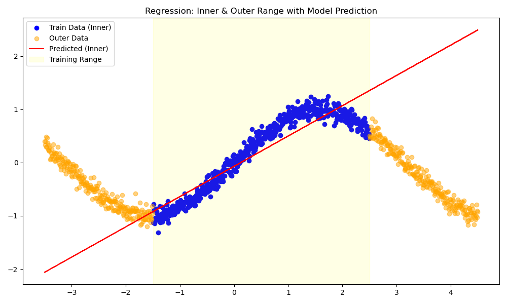
Figure: Fitting a sine wave with a single linear neuron.
Adding Nonlinearity: ReLU
Adding a ReLU activation gives us a “kink,” but still only allows for piecewise linear fits:
f(x) = \max(0, x)
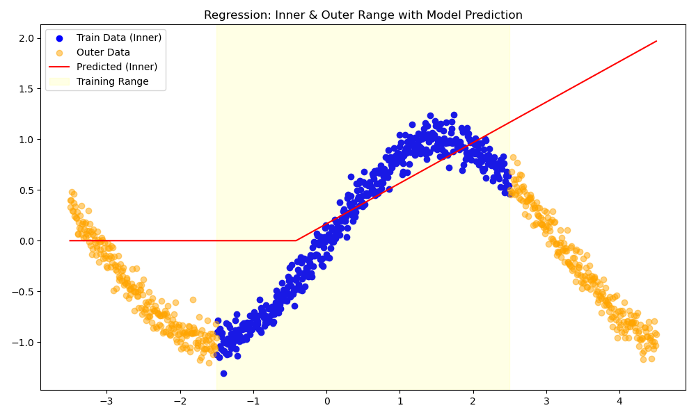
Figure: Fitting a sine wave with a single ReLU neuron.
More Neurons, More Segments
What if we used two neurons in a hidden layer with ReLU activations? Now we can fit a piecewise linear function with two segments:
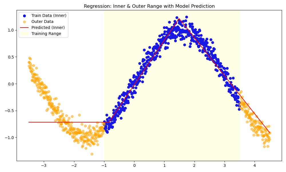
By adding more neurons, the network can fit more piecewise linear segments, but it’s not able to accommodate smooth curves, like a sine wave. The network is fundamentally limited by the linearity of each segment.
It is common to include functions that have curves, e.g. using a tanH activation function instead of ReLU. However, these are typically only implemented in the final output layer.
Key Takeaways
- Single linear neuron: fits a straight line.
- Single ReLU neuron: fits a line with a kink.
- Multiple ReLU neurons: fits a piecewise linear function.
- Generalization: Even with more neurons, the network struggles to extrapolate or capture smooth nonlinearities outside the training region.
PyTorch builds complexity by stacking simple layers, not by fitting high-order polynomials directly. Understanding these basics helps explain both the power and the limitations of neural networks.
Discussion
Neural networks are powerful because they combine many simple units. However, each unit has inherent limitations. Understanding these limits is crucial for building intuition about what your models can and cannot learn, and why extrapolation is often unreliable.
This highlights some fundamental concepts that are often overlooked in the rush to build complex models:
-
Piecewise Linear Nature:
Neural networks are fundamentally based on piecewise approximations of small linear segments. The more neurons and layers you add, the more complex the piecewise function becomes. However, at each layer, the transformations are still linear in nature. This limitation is important to keep in mind when interpreting the capabilities of your model. -
Training Range Limitations:
Neural networks can only reliably predict values within the range of the data they were trained on. Extrapolation beyond the training data is inherently unreliable. This raises an important question:
What is the range of the data when dealing with images, high-dimensional data, or language data?
Defining the range of such data in a meaningful way is a challenging and often philosophical problem.
While state-of-the-art neural networks can achieve remarkable feats—such as passing a Turing test, it’s important to remember that they are approximations of the underlying functions they are trying to model. This has significant implications for how we interpret their outputs and understand their limitations in generalization.
(But they are REALLY good approximations!)
Thought Experiment:
“If you give an AI enough information about an elephant, does it implicitly know about a cat?”
— Someone, somewhere on the internet (probably)
No.
This simple thought experiment underscores the importance of understanding the limitations of neural networks. They do not “know” or “understand” concepts outside the scope of their training data, they approximate patterns within the data they’ve seen.
In Part 3, we’ll explore how to scale up these concepts with PyTorch Lightning, focusing on abstraction and the ongoing challenge of hyperparameter tuning.